Statistical Quality
A variety of statistical metrics and techniques can be used to compare the original and synthetic data distributions.
These can be used to assess the synthetic data and its statistical resemblance to the original data. Each of these
metrics are available in synthesized.insight.metrics.
Univariate Metrics
The distributions of each column in the original and synthesized dataset (of both continuous and categorical attributes) are compared using univariate statistical distance metrics. For each attribute in the data, these provide a comparison of the marginal probability distributions of the original and synthetic data. The following metrics are available:
-
EarthMoversDistance: calculates the Earth Mover’s distance (also known as the 1-Wasserstein distance) between two categorical attributes. -
KolmogorovSmirnovDistance: calculates the Kolmogorov-Smirnov statistic between two continuous attributes.
Both of these distances vary between 0.0 and 1.0, where a value of 0.0 occurs when the original and synthetic data have exactly identical distributions. These metrics can be applied to compare the individual attributes of the synthetic and original data.
from synthesized.insight.metrics import EarthMoversDistance

df_synth = synthesizer.synthesize(1000)
emd = EarthMoversDistance()
emd(df_original['categorical_column'], df_synth['categorical_column'])
Interaction Metrics
Beyond univariate measures that look at single attributes in isolation, correlations and associations between each column can also be measured and compared between the synthetic and original datasets. Several metrics are used depending on whether the attributes to compare are categorical or continuous:
-
KendallTauCorrelation: calculates the Kendell-Tau coefficient. This measures the correlation between two ordinal continuous attributes. (Note: this assumes the two variables have a monotonic relationship.) -
CramersV: calculates the Cramer’s V value. This measures the strength of the association between two categorical attributes. -
CategoricalLogisticR2: calculates McFadden’s R squared. This measures the association between a categorical and continuous attribute. -
SpearmanRhoCorrelation: calculates Spearman’s rank correlation coefficient. This measures the association between two ordinal continuous attributes. (Note: this assumes the two variables have a monotonic relationship.)
Each of these metrics can be calculated on the original and synthetic data, and then compared to determine their statistical similarity.
from synthesized.insight.metrics import CramersV

df_synth = synthesizer.synthesize(1009)
cramers = CramersV()

# calculate association on original data
cramers(df_original["categorical_column_a"], df_original["categorical_column_b"])

# calculate association on synthetic data
cramers(df_synth["categorical_column_a"], df_synth["categorical_column_b"])
These metrics check the input data to ensure it is categorical or continuous, depending on the assumptions of the
metric. If the data is of the incorrect type they will return None.
|
Assessor
Alternatively, the evaluation metrics can be automatically calculated and visualized for the synthetic and original
data sets using the Assessor class.
Assessor requires a DataFrameMeta class extracted from the
original data-frame, and can be created with these commands:
from synthesized import MetaExtractor
from synthesized.testing import Assessor

df_meta = MetaExtractor.extract(df)
assessor = Assessor(df_meta)
Once the Assessor, it can be used to compare marginal distributions, joint distributions,
and classification metrics between two data-frames, usually the original and generated data-frames(df_orig
and df_synth).
Comparing Marginal Distributions
show_distributions plots all marginal distributions in two datasets,
assessor.show_distributions(df_orig, df_synth)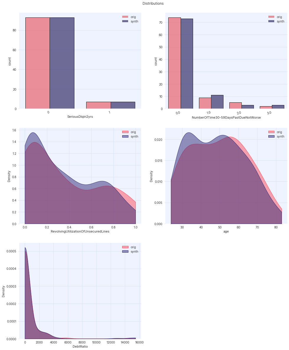
Example plot for assessor.show_distributions().
assessor.show_ks_distances() and assessor.show_emd_distances() plot for each column the
KolmogorovSmirnovDistance and EarthMoversDistance difference between both datasets:
assessor.show_ks_distances(df_orig, df_synth)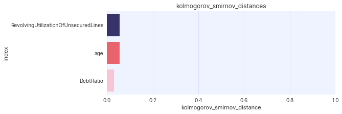
Example plot of assessor.show_ks_distances().
The user can also plot the difference of any other univariate metric (let’s call it MyDistanceMetric) with the
following command:
assessor.show_first_order_metric_distances(MyDistanceMetric())Comparing Joint Distributions
The Assessor class is also able to plot different joint distributions and correlation distances in two
different manners:
-
show_second_order_metric_matricesplots the matrices of all combinations of columns, with the value of the specified metric between each pair columns in the corresponding cell. -
show_second_order_metric_distancesplots the distance of the given metric for each pair of columns between both datasets.
Both functions are available for the four interaction metrics defined above. For example;
assessor.show_kendall_tau_distances(df_orig, df_synth)
assessor.show_spearman_rho_matrices(df_orig, df_synth)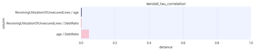
Example plot of assessor.show_kendall_tau_distances().
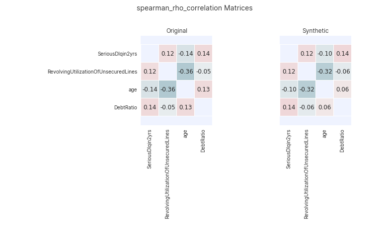
Example plot of assessor.show_spearman_rho_matrices().