Time-Series Synthesis
|
The full source code for this example is available for download here along with the example dataset. |
Prerequisites
This tutorial assumes that you have already installed the Synthesized package. While it is not required to have read the single table synthesis tutorial, it is highly recommended that you do so, as it outlines best practices when generating and evaluating synthetic data. It is assumed that you are also familiar with the format of a time-series dataset as laid out in the documentation.
Introduction
In this tutorial, the TimeSeriesSynthesizer is introduced as a means to generate data while maintaining the temporal
correlations present in the original dataset. In particular, the focus will be on time-series data where there is a
regular time interval between measurements.
This example explains the format of a time-series dataset and how it relates to creating an instance of the TimeSeriesSynthesizer.
The ability to train a TimeSeriesSynthesizer with a custom configuration is also demonstrated.
Financial Dataset
This tutorial will use an example dataset of one hundreds day’s worth of stock information of a subset of 25 companies in the S&P 500:
import pandas as pd
df = pd.read_csv("sp_500_subset.csv")
df
Name date open high low close volume GICS Sector 0 ALK 2013-02-08 23.995 24.435 23.940 24.335 1013314 Industrials 1 ALK 2013-02-11 24.410 24.603 24.120 24.400 1124948 Industrials 2 ALK 2013-02-12 24.405 24.560 24.270 24.430 1280160 Industrials 3 ALK 2013-02-13 24.440 24.760 24.385 24.760 1146758 Industrials 4 ALK 2013-02-14 24.665 24.680 24.150 24.355 1205950 Industrials ... ... ... ... ... ... ... ... ... 2495 WHR 2013-06-26 114.850 116.730 111.940 112.550 1226273 Consumer Discretionary 2496 WHR 2013-06-27 113.720 116.000 112.530 115.430 898379 Consumer Discretionary 2497 WHR 2013-06-28 115.310 115.740 114.060 114.360 1137362 Consumer Discretionary 2498 WHR 2013-07-01 115.550 117.760 114.540 115.900 884096 Consumer Discretionary 2499 WHR 2013-07-02 116.010 117.950 115.670 116.350 1150999 Consumer Discretionary [2500 rows × 8 columns]
This dataset is regular and not event-based as there is a constant interval between measurements of one business day.
Currently the TimeSeriesSynthesizer requires that measurements are taken over identical time-periods for every
unique entity, i.e. measurements should start and end on the same day, and the interval should be the same for each
set of time-series data across the whole dataset.
|
This tutorial will demonstrate how the SDK can be used to generate data for new companies, over the same time period, which are statistically similar to the types of companies present in the original dataset. Such a task has real-world applicability in scenarios where:
-
Original data is not available past a certain date, or at all
-
Data volume is low
As described in the single table synthesis tutorial, it is best practice to perform EDA prior to generating any new data, with the downstream task in mind. This ensures that the relevant metrics can be tested when evaluating the quality of the generated data. If you have not already read the single table synthesis tutorial you are highly recommended to do so.
Synthesis
The workflow for producing time-series data is slightly different from that when producing tabular data because of a
number of preprocessing steps that occur under-the-hood. For example, rather than first performing a meta extraction and
creating the model with the resulting meta object, the meta extraction is handled by the TimeSeriesSynthesizer
itself. The reason for this is that a time-series dataset is formed of data from multiple entities, as outlined in
our documentation concerning Time-Series Synthesis, and needs to be preprocessed before meta extraction
occurs. This preprocessing ensures, amongst other things, that each unique entity has the same number of time steps in
the dataset (see the above note). Only after this preprocessing can the meta data be extracted.
In order to train the model with the desired number of time steps we need to specify max_time_steps in
DeepStateConfig, used to configure the underlying model. The max_time_steps argument controls
the maximum number of time steps to process from each unique entity. By default this is set to 100.
from synthesized.config import DeepStateConfig
config = DeepStateConfig(max_time_steps=100)
The DeepStateConfig instance can then be passed to the TimeSeriesSynthesizer upon model creation, along with the
original dataset and the time-series column specification:
from synthesized import TimeSeriesSynthesizer

id_idx = "Name"
time_idx = "date"
event_cols=["open", "high", "low", "close", "volume"]
const_cols=["GICS Sector"]

synth = TimeSeriesSynthesizer(
    df,
    id_idx=id_idx,
    time_idx=time_idx,
    event_cols=event_cols,
    const_cols=const_cols,
    exog_cols=None,
    associations=None,
    config=config
)
synth.learn(epochs=20, steps_per_epoch=500)
Note that since the TimeSeriesSynthesizer handles the process of meta extraction, associations are passed through as an argument upon
instantiation. For more information on Associations see our documentation.
|
The preprocessing carried out by the |
Having trained the model we are now in a position to synthesize a new sequence of time-series data, however there are
additional positional arguments that can be specified when using the TimeSeriesSynthesizer, compared to the
HighDimSynthesizer, that can generate synthetic time-series data for specific unique entities, or over specific
time-periods.
-
n: The total number of time-steps to synthesize. -
df_exogenous: Exogenous variables linked to the time-series. Must have the same number of rows as the valuen. Currently this argument must be provided for regular time-series synthesis. Note that theTimeSeriesSynthesizeralso treats the column specified bytime_idxas an exogenous variable during synthesis. -
id: This optional argument can be used to specify the unique ID of the sequence. If provided, it must correspond to an ID in the raw dataset used during training. If this argument is not specified then time-series data corresponding to a new ID is generated. -
df_const: Constant values linked to the givenid. This should be a DataFrame containing a single row of values, where the columns correspond to those given inconst_colson instantiating theTimeSeriesSynthesizer. Ifidis provided andconstant_colswas defined in the initialization then this argument should also be specified. -
df_time_series: Time series measurements linked to the givenid. Providingdf_time_seriescan influence the underlying deep generative engine to generate a particular initial state that is then used during time-series generation. The provided DataFrame must contain the same columns specified inevent_cols. Any number of rows ≤ncan be provided.
For example, the trained TimeSeriesSynthesizer object can be used to generate data representative of a single company "HCA"
for a period of 100 business days, using the first 50 days of that company’s real data to influence the underlying
deep generative engine with the df_time_series argument
df_hca = df.set_index(id_idx).xs("HCA").head(100).reset_index()

df_synth = synth.synthesize(
    n=100,
    id="HCA",
    df_const=df_hca[const_cols].head(1),
    df_exogenous=df_hca[[time_idx]],
    df_time_series=df_hca[event_cols].head(50)
)
df_synth
Name date open high low close volume GICS Sector 0 HCA 2013-02-08 36.694706 37.038177 36.078388 36.538799 1860650 Health Care 1 HCA 2013-02-11 36.808865 37.253441 36.351429 36.785351 5322930 Health Care 2 HCA 2013-02-12 35.848190 36.524796 35.500824 36.112301 6412000 Health Care 3 HCA 2013-02-13 35.556534 35.876644 35.001110 35.394936 6360522 Health Care 4 HCA 2013-02-14 35.594650 35.987000 35.175346 35.500397 4425438 Health Care ... ... ... ... ... ... ... ... ... 95 HCA 2013-06-26 34.318676 34.621418 33.888035 34.346100 4049286 Health Care 96 HCA 2013-06-27 33.530663 33.962631 32.983322 33.385921 7207552 Health Care 97 HCA 2013-06-28 32.895248 33.251427 32.501842 32.746380 10017537 Health Care 98 HCA 2013-07-01 34.704765 35.062428 34.193974 34.652153 4976035 Health Care 99 HCA 2013-07-02 32.865849 33.208466 32.468525 32.651272 2631518 Health Care [100 rows × 8 columns]
The TimeSeriesAssessor (a subclass of the Assessor class capable of handling
data with a temporal component) can be used to plot the features of the original and generated time series alongside one another for a
quick comparison:
from synthesized.testing import TimeSeriesAssessor
assessor = TimeSeriesAssessor(synth, df_hca, df_synth)
assessor.show_series(columns=["volume"])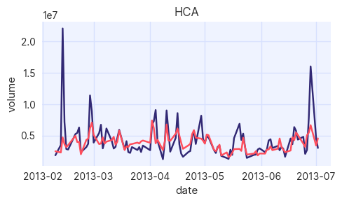
A more complex method of evaluating statistical quality is to compare to the auto-correlations of the synthetic and original data. Simply put, the auto-correlation is a measure of how correlated a signal is with itself at some future time step.
assessor.show_auto_associations(columns=["volume"])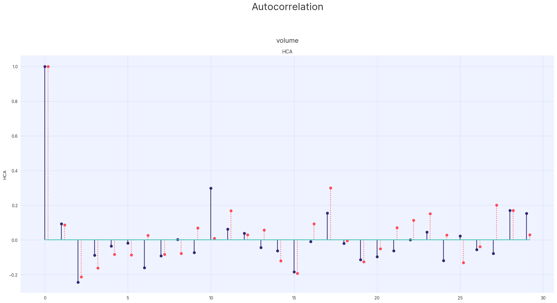
Since the TimeSeriesAssessor subclass the Assessor class, it is possible to analyse the univariate and bivariate
relationships present in the data.
|
Analysing the univariate and bivariate relationships across the whole dataset will lead to aggregate statistics that may lack any real utility. Since a time-series dataset is made up of many unique entities you should analyse each unique entity separately or analyse groups of similar entities. This is demonstrated below where entities in the same industry are compared to one another. |
As described in the single table tutorial, it is best practice to run an end-to-end synthesis using
the default parameters of the SDK. Following an initial evaluation of the data from this first iteration, fine-tuning can
be performed in order to optimise for particular metrics. For more information on fine-tuning the TimeSeriesSynthesizer
training please see the hyperparameter tuning tutorial.
Synthesize New Entities
In order to generate new entities, the id argument is not specified in the call to the synthesize method. Instead,
the TimeSeriesSynthesizer will generate data corresponding to a completely new entity. Two simple functions, generate_id()
and synthesize_with_generated_id() can then be used to create data for as many new companies as desired.
import random
from string import ascii_uppercase

def generate_id(length):
    return "".join(random.sample(ascii_uppercase, length))

def synthesize_with_generated_id(synth, time_steps, num_companies, df_exogenous):
    df_synth = []
    for _ in range(num_companies):
        df_temp = synth.synthesize(time_steps, df_exogenous=df_exogenous)
        df_temp[id_idx] = generate_id(random.choice([3, 4]))
        df_synth.append(df_temp)

    return pd.concat(df_synth)

num_rows = synth.max_time_steps
df_synth = synthesize_with_generated_id(synth, num_rows, 25, pd.DataFrame({time_idx: pd.bdate_range(start="2013-02-08", periods=num_rows, freq="B")}))
df_synth
Name date open high low close volume GICS Sector 0 XWVK 2013-02-08 65.079063 66.157959 64.145058 64.720009 1171235 Consumer Staples 1 XWVK 2013-02-11 66.344330 67.218124 65.565895 66.089142 1147964 Consumer Staples 2 XWVK 2013-02-12 62.074646 62.686962 61.499718 62.006413 1592895 Consumer Staples 3 XWVK 2013-02-13 60.428658 60.974365 59.905689 60.468658 1250439 Consumer Staples 4 XWVK 2013-02-14 57.723057 58.188950 57.130550 57.587269 1666838 Consumer Staples ... ... ... ... ... ... ... ... ... 2495 IUBF 2013-06-21 40.939720 41.385315 40.312225 40.804897 3962583 Information Technology 2496 IUBF 2013-06-24 41.417465 41.660675 40.833221 41.296997 2556655 Information Technology 2497 IUBF 2013-06-25 41.736416 42.317898 41.360413 41.895920 2385364 Information Technology 2498 IUBF 2013-06-26 41.401161 41.662865 40.916771 41.239063 2788163 Information Technology 2499 IUBF 2013-06-27 44.183121 44.649666 43.810211 43.990318 4173762 Information Technology [2500 rows × 8 columns]
In the above example the relatively simple generate_id() method creates a new company name by sampling from the 26 characters of the alphabet.
It is possible to generate more complex ID’s for different purposes using the SDK’s Entity Annotations.
Once again, it is instructive to perform a quick visual check of the generated data. It is a reasonably safe assumption that companies from the same industry will perform relatively similarly, therefore a plotting function is defined that compares original and synthetic companies from the same industry against one another:
import seaborn as sns

def plot_by_industry(df_orig, df_synth, column, industry):

    df_orig_industry = df_orig.set_index("GICS Sector").xs(industry).reset_index()
    df_synth_industry = df_synth.set_index("GICS Sector").xs(industry).reset_index()

    df_comparison = pd.concat([df_orig_industry.assign(src="orig"), df_synth_industry.assign(src="synth")], axis=0, ignore_index=True)

    g = sns.relplot(df_comparison, x=time_idx, y=column, hue=id_idx, col="src", kind="line", legend=False)
    g.fig.suptitle(f"{industry}", fontsize=16)
    g.fig.subplots_adjust(top=0.9);

df[time_idx] = pd.to_datetime(df[time_idx])

for industry in df_synth["GICS Sector"].unique():
    plot_by_industry(df, df_synth, "volume", industry)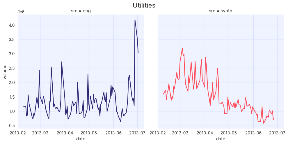
Quickly scanning the results, it is clear that the TimeSeriesSynthesizer is producing data on the same scale as the
original data for each company. The volatility (a measure of how data deviates from short term averages) of the synthetic
data for each industry also bears resemblance to the original.
In addition to the metrics described in the single table tutorial, it can be helpful to analyse the aggregate statistics across time series data:
def aggregate(df_orig, df_synth, stat, col):

    agg_statistic = {}

    for industry in df_synth["GICS Sector"].unique():
        agg_statistic[industry] = [
            getattr(df_orig.set_index("GICS Sector").xs(industry)[col], stat)(),
            getattr(df_synth.set_index("GICS Sector").xs(industry)[col], stat)(),
        ]
    return pd.DataFrame(data=agg_statistic, index=[f"orig_{stat}", f"synth_{stat}"])
such as the mean:
aggregate(df, df_synth, "mean", "volume")Consumer Industrials Real Estate Tech Health Utilities Consumer Finance Energy Materials orig_mean 1882369.39 2.669255e+06 601194.23 4.849214e+06 3692133.22 1334860.62 3.449932e+06 1680161.76 3830912.86 1626211.45 synth_mean 2609669.50 1.782956e+06 1252000.13 6.262940e+06 1330549.92 1129092.86 1.679943e+06 1376112.13 1235479.45 1226837.30
and standard deviation:
aggregate(df, df_synth, "std", "volume")Consumer Industrials Real Estate Tech Health Utilities Consumer Finance Energy Materials orig_std 1.071113e+06 3.243124e+06 493193.509604 3.430623e+06 2.756140e+06 571058.30515 4.000987e+06 790336.061546 1.297486e+06 715367.615106 synth_std 1.739509e+06 9.652454e+05 460453.034697 4.328634e+06 4.615111e+05 277333.09643 8.058934e+05 575133.707806 4.096204e+05 404923.338977
It is expected that there are deviations between the values of the aggregate metric in the original and synthetic data,
both due to the relatively small numbers of companies in particular industries and due to the nature of how the TimeSeriesSynthesizer
generates data.
As described in the single table tutorial, the utility of synthetic data can be analysed from three angles:
-
Statistical Quality
-
Predictive Utility
-
Privacy
The simple analysis laid out above can be classified as an evaluation of the statistical quality of the data, but it is by no means exhaustive. Analysing time series data is a complex subject, and should be informed by the downstream use cases the data will be applied to.