Rebalancing
|
The full source code for this example is available for download here. |
Prerequisites
This tutorial assumes that you have already installed the Synthesized package and have an understanding how to use the tabular synthesizer. If you are new to Synthesized, we recommend you start with the quickstart guide and/or single table synthesis tutorial before jumping into this tutorial.
Introduction
In this tutorial we will demonstrate how to the SDK can be used to alter the distributions of a dataset. This is useful if the user wants to reshape their data for a specific purpose. For example, the user may have a dataset with a target column that is extremely imbalanced. The user may want to train a classification model to try and predict the value of the target column, but because of the imbalance in the target column, the model may not perform well. Using the technique of data rebalancing, the dataset can be reshaped to improve the performance of the classification model.
In this tutorial we will walk through an explicit example where data rebalancing is used to improve the performance of a classification model trained on an originally highly imbalanced dataset.
For more information on the techniques used in this tutorial, and an in-depth discussion on reducing data bias using these techniques, see our blog post or the documentation.
Credit Dataset
In this tutorial we will use a public credit scoring dataset from Kaggle,
also available with the synthesized_datasets package:
import synthesized_datasets
import pandas as pd

df_orig = synthesized_datasets.CREDIT.credit.load()
df_orig
SeriousDlqin2yrs RevolvingUtilizationOfUnsecuredLines age ... NumberOfTime60-89DaysPastDueNotWorse NumberOfDependents 0 1 0.766127 45 ... 0 2.0 1 0 0.957151 40 ... 0 1.0 2 0 0.658180 38 ... 0 0.0 3 0 0.233810 30 ... 0 0.0 4 0 0.907239 49 ... 0 0.0 ... ... ... ... ... ... ... 149995 0 0.040674 74 ... 0 0.0 149996 0 0.299745 44 ... 0 2.0 149997 0 0.246044 58 ... 0 0.0 149998 0 0.000000 30 ... 0 0.0 149999 0 0.850283 64 ... 0 0.0 [150000 rows x 11 columns]
The binary classification column "SeriousDlqin2yrs", denoting whether someone has defaulted on a loan within the last 2 years, will be the target variable. The remaining columns will be explanatory variables that will be used to train a classification model.
y_label = "SeriousDlqin2yrs"
x_labels = [col for col in df_orig.columns if col != y_label]
The target column is highly imbalanced. This can be seen by looking at the value counts of the target column:
value_counts = df_orig[y_label].value_counts()
value_counts
0 139974 1 10026 Name: SeriousDlqin2yrs, dtype: int64
Plotting the value counts of the target column shows the imbalance more clearly:
pd.cut(df_orig[y_label],
       bins=[-0.5, 0.75, 1],
       labels = ['0','1'])\
  .value_counts(sort=False).plot.bar()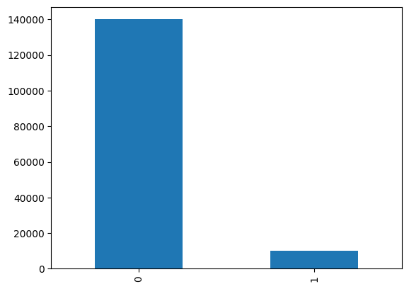
We see that approximately 93% of the rows in the dataset have a value of 0 for the target column, and only 7% have a value of 1.
Training a Linear Classification Model
In the following, a linear RidgeClassifier model will be used to try and predict the value of the target variable
SeriousDlqin2yrs. The remainder of the columns are used as explanatory variables.
The test-train-split technique will be used to evaluate the performance of the model in that task.
Before fitting the RidgeClassifier model some preprocessing needs to be applied to the dataset.
The SDK offers the preprocess() convenience function that will be used to preprocess the dataset. The preprocessing will
label, or one-hot encode the categorical columns, and transform the continuous columns using a StandardScaler.
from synthesized.insight.modelling import ModellingPreprocessor

def preprocess(
    df: pd.DataFrame,
    preprocessor: ModellingPreprocessor
):
    df_processed = preprocessor.transform(df)
    y = df_processed.pop(preprocessor.target).to_numpy()
    x = df_processed.to_numpy()
    return x, y
In the first instance, the RidgeClassifier will be trained on the original data:
from sklearn.model_selection import train_test_split

test_size = 0.2

df_train, df_test = train_test_split(
    df_orig,
    test_size=test_size,
    stratify=df_orig[y_label],
    random_state=42,
)

preprocessor = ModellingPreprocessor(target=y_label)
preprocessor.fit(df_orig)

x_train, y_train = preprocess(df_train, preprocessor)
x_test, y_test = preprocess(df_test, preprocessor)
The RidgeClassifier model will be fitted using the train subset of the data:
from sklearn.linear_model import RidgeClassifier
orig_classifier = RidgeClassifier()
orig_classifier.fit(x_train, y_train)
The ability of the model to classify unseen data will then be evaluated using the test subset:
y_predict = orig_classifier.predict(x_test)The area under the ROC-curve (ROC-AUC) is used to evaluate the performance of the model in classifying the unseen test data. The value of the ROC-AUC varies between 0 and 1, with 1 implying perfect separability between the two classes , and 0 implying the model predicts the exact incorrect class for each row. A value of 0.5 means that the model hasn’t learnt any difference between the classes, and has no predictive capacity.
from sklearn.metrics import roc_auc_score
orig_roc_auc = roc_auc_score(y_test, y_predict)
orig_roc_auc
0.5703505568994107
The value of ~0.57 implies that the model has some predictive capacity, but not much better than a random guess.
Using Rebalanced Synthetic Data
The performance of the linear RidgeClassifier model in the previous section was, on the whole, pretty poor. The
reasoning can be traced back to the data used to train the model: the high imbalance in the target column means that
the class 1 in the target column has a very faint signal.
A naive solution to this problem is to create a new dataset by oversampling data from the minority class and undersampling from the majority in order to achieve the desired distribution of classes. However, there is a very clear drawback to this method in that the new dataset may be significantly smaller than the original. Using this traditional technique, the issue has been transformed from not having enough quality data to potentially not having enough data at all.
More advanced methods, such as SMOTE, create entirely new data points for the minority class to augment the original dataset with. The downside of SMOTE is that there is no understanding of the statistics of the original data meaning that the correlations between variables is lost, degrading model performance.
Alternatively, the deep generative models utilised in the HighDimSynthesizer can be used to learn the statistical
properties and correlations present in the original data and synthesize a dataset containing columns adhering to user
defined distributions.
To generate the synthetic data we first create a HighDimSynthesizer instance using the meta data extracted from the
original dataset:
from synthesized import HighDimSynthesizer, MetaExtractor
df_meta = MetaExtractor.extract(df_orig)
synth = HighDimSynthesizer(df_meta)
The HighDimSynthesizer instance is then trained using the train subset of the original that was defined above - the
test subset is held back to prevent any possible data leaks.
synth.learn(df_train)Rather than simply calling the HighDimSynthesizer.synthesize() method, the ConditionalSampler class can be used
to generate completely new, synthetic data where the proportions of the two classes in the target variable have been
rebalanced to occur in equal proportions.
An instance of the ConditionalSampler can be created by passing in a trained instance of the HighDimSynthesizer.
To generate rebalanced data, the desired distributions of the classes in the target column are specified using the
explicit_marginals argument of the sample() method:
from synthesized import ConditionalSampler
sampler = ConditionalSampler(synth)
explicit_marginals = {y_label: [(0, 0.5), (1, 0.5)]}
df_synth = sampler.sample(
    num_rows=len(df_train),
    explicit_marginals=explicit_marginals,
    max_trials=40
)
To verify that the distribution of the target column has indeed been rebalanced, the
Assessor module can be used to visually inspect the distributions of the
variables in the synthetic data compared to the original.
from synthesized.testing import Assessor
assessor = Assessor(df_meta)
assessor.show_distributions(df_train, df_synth);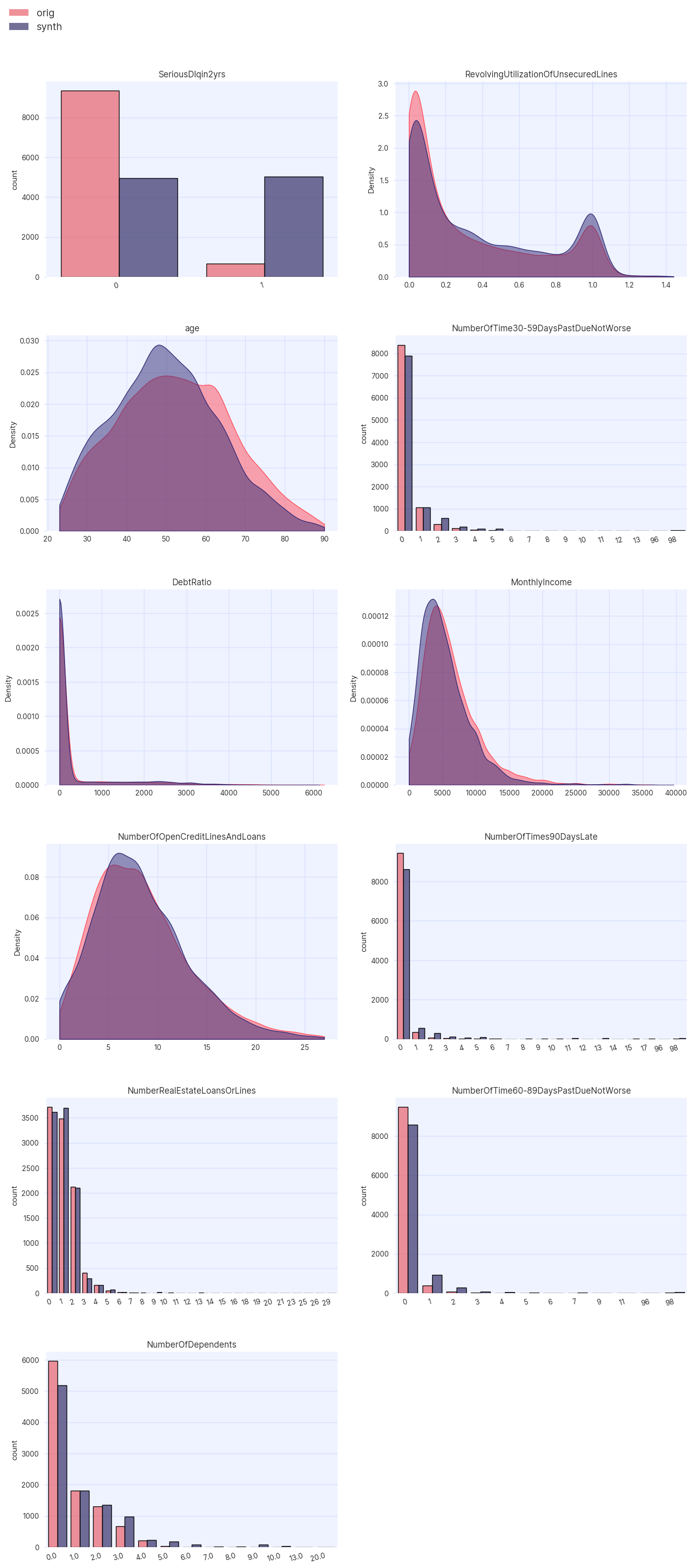
As demonstrated in the distributions, the target variable has been rebalanced such that the classes now appear in equal proportions (50% each).
The rebalancing of the target variable has also had an effect on the distributions of the other variables in the dataset.
This is because correlations between variables are learnt by the HighDimSynthesizer and are used to generate the rebalanced synthetic data.
For example, the peak of the age distribution has been shifted to the left, implying that younger
individuals may be more likely to default.
The training of a RidgeClassifier model can now be conducted using the rebalanced synthetic dataset as the training data.
For fairness of comparison, the same test dataset will be used to evaluate the performance of this model as was used when
evaluating the performance of the model trained with original data. It is important to note that synthetic data should never
be used as test data and should only be used when training the model of interest.
preprocessor = ModellingPreprocessor(target=y_label)
preprocessor.fit(pd.concat([df_orig, df_synth]))

x_synth, y_synth = preprocess(df_synth, preprocessor)

synth_classifier = RidgeClassifier()
synth_classifier.fit(x_synth, y_synth)

y_predict = synth_classifier.predict(x_test)
Again, using the ROC-AUC as a metric of model performance, we see an enormous increase in the new models ability to distinguishing the two classes when compared with the original model:
synth_roc_auc = roc_auc_score(y_test, y_predict)
synth_roc_auc
0.7306853423683158
Because synthetic data in the SDK is generated from random noise, if new set of synthetic data were generated, and a linear model is trained with the resulting dataset we would observe that the ROC-AUC would fluctuate around a mean value.
synth_roc_auc / orig_roc_auc1.2811162074435958
By comparing the ROC-AUC of the model trained with synthetic data to the model trained with original data, we see that the new model displays a 25 - 30% improvement in performance.
Bootstrapping Original Data
In the above, we used rebalanced, purely synthetic data to train a linear classification model. However, the
ConditionalSampler offers an alternative means to generate rebalanced data by augmenting the original data with
synthetic data composed of the minority class using the alter_distributions() method.
The same ConditionalSampler instance created above will be used, but we will configure it to generate a dataset containing a
mixture of real and synthetic data.
When creating such a dataset, care must be taken when performing the test/train split. As mentioned above, it is important to ensure that no synthetic data is used to test the model, therefore only the distributions of the train dataset should be altered.
explicit_marginals = {y_label: [(0, 0.5), (1, 0.5)]}
df_altered = sampler.alter_distributions(
    df_train,
    num_rows=len(df_train),
    explicit_marginals=explicit_marginals,
    max_trials=40
)

x_altered, y_altered = preprocess(df_altered, preprocessor)

altered_classifier = RidgeClassifier()
altered_classifier.fit(x_altered, y_altered)

y_predict = altered_classifier.predict(x_test)

altered_roc_auc = roc_auc_score(y_test, y_predict)
altered_roc_auc
0.7356642328809161
Using bootstrapped data, we see a very similar ROC-AUC score to when we trained the model with purely synthetic data.